dunnhumby Consumer Data: Customer Lifetime Value

Introduction

In my last post, we used k-means clustering to create customer segments. Customers were grouped into these segments to be able to better meet individual customers’ needs. We specifically looked at customer loyalty which was measured using a mix of recency, frequency, and value (RFV).

Next, we are going to take these customer loyalty segments, along with our transactional data, and predict customer lifetime value.

Customer Lifetime Value

Customer lifetime value (CLV) is pretty straightforward, it’s the amount of money that a customer is expected to spend on your product(s) during their lifetime.

When a business knows how much a customer is worth to them, it helps with decisions regarding customer retention. If a customer has a lifetime value of $100, then a business would not want to spend any more than that to try to keep their business. Spending more than $100 to retain this customer would result in losing money. However, if a customer has a lifetime value of $100,000, then the business may be willing to spend tens of thousands of dollars to try to retain the customer’s business.

CLV can also be used with customer acquisition decisions. If you predict the CLV for a certain type of customer, then you know how much money you would be willing to spend to acquire that customer and still turn a profit.

Analytical Framework

Data Preparation

The dunnhumby dataset that we have been analyzing spans 102 weeks. During the exploratory data analysis, it was found that the first 4 months of data weren’t consistent with the rest, so we have been excluding those 4 months from our analyses. That leaves us with roughly a year and a half of data.

For the purposes of this project, a customer’s “lifetime” will be defined as one year (52 weeks). We will build a model to predict customer lifetime value using the 26 weeks (half of a year) immediately preceding.

To do this, the feature set will be made up of all customer transactional data from weeks 24 to 50. The dependent variable our model will be trained on will be customer revenue in weeks 51 – 102 (this is how we are measuring CLV).

Below is the code used to create our feature set as previously described. We will be defining customer loyalty segments for our 26-week feature set using the same method that we used in the previous Customer Segmentation post. Be sure to check it out now, if you haven’t already.

trans_26wk <- transaction_data[transaction_data$WEEK_NO >= 24 & transaction_data$WEEK_NO <= 50,]
trans_52wk <- transaction_data[transaction_data$WEEK_NO >= 51,]

# RFV for 26wk data

# Recency
max_day <- max(trans_26wk$DAY)

recency_table_26wk <- trans_26wk %>%
  group_by(household_key) %>%
  summarise(MaxPurchaseDate = max(DAY),
            Recency = max_day - max(DAY))

# recency plot
ggplot(data=recency_table_26wk, aes(x=Recency)) +
  geom_histogram()

# kmeans cluster into 4 groups
set.seed(1234)
recency_k <- kmeans(recency_table_26wk$Recency, centers = 4)
recency_table_26wk$Cluster <- recency_k$cluster
recency_table_26wk$Score <- ifelse(recency_table_26wk$Cluster==1,1,
                              ifelse(recency_table_26wk$Cluster==3,2,
                                     ifelse(recency_table_26wk$Cluster==4,3,4)))


# Frequency
frequency_table_26wk <- trans_26wk %>%
  group_by(household_key) %>%
  summarise(Frequency = length(unique(BASKET_ID)))

# frequency plot
ggplot(data=frequency_table_26wk, aes(x=Frequency)) +
  geom_histogram()

# kmeans cluster into 4 groups
set.seed(1234)
frequency_k <- kmeans(frequency_table_26wk$Frequency, centers = 4)
frequency_table_26wk$Cluster <- frequency_k$cluster
frequency_table_26wk$Score <- ifelse(frequency_table_26wk$Cluster==3,1,
                                     ifelse(frequency_table_26wk$Cluster==4,2,
                                            ifelse(frequency_table_26wk$Cluster==1,3,4)))


# Revenue
revenue_table_26wk <- trans_26wk %>%
  group_by(household_key) %>%
  summarise(Revenue = sum(REVENUE))

# revenue plot
ggplot(data=revenue_table_26wk, aes(x=Revenue)) +
  geom_histogram()

# kmeans cluster into 4 groups
set.seed(1234)
revenue_k <- kmeans(revenue_table_26wk$Revenue, centers = 4)
revenue_table_26wk$Cluster <- revenue_k$cluster
revenue_table_26wk$Score <- ifelse(revenue_table_26wk$Cluster==3,1,
                              ifelse(revenue_table_26wk$Cluster==4,2,
                                     ifelse(revenue_table_26wk$Cluster==1,3,4)))


# Customer Profiles
customer_profiles_26wk <- cbind(recency_table_26wk$household_key,
                           recency_table_26wk$Recency,
                           recency_table_26wk$Score,
                           frequency_table_26wk$Frequency,
                           frequency_table_26wk$Score,
                           revenue_table_26wk$Revenue,
                           revenue_table_26wk$Score)
customer_profiles_26wk <- as.data.frame(customer_profiles_26wk)
colnames(customer_profiles_26wk) <- c("household_key",
                                 "Recency",
                                 "RecencyCluster",
                                 "Frequency",
                                 "FrequencyCluster",
                                 "Revenue",
                                 "RevenueCluster")
customer_profiles_26wk$household_key <- as.character(customer_profiles_26wk$household_key)
customer_profiles_26wk$Recency <- as.numeric(as.character(customer_profiles_26wk$Recency))
customer_profiles_26wk$RecencyCluster <- as.numeric(as.character(customer_profiles_26wk$RecencyCluster))
customer_profiles_26wk$Frequency <- as.numeric(as.character(customer_profiles_26wk$Frequency))
customer_profiles_26wk$FrequencyCluster <- as.numeric(as.character(customer_profiles_26wk$FrequencyCluster))
customer_profiles_26wk$Revenue <- as.numeric(as.character(customer_profiles_26wk$Revenue))
customer_profiles_26wk$RevenueCluster <- as.numeric(as.character(customer_profiles_26wk$RevenueCluster))

customer_profiles_26wk$OverallScore <- customer_profiles_26wk$RecencyCluster + customer_profiles_26wk$FrequencyCluster + customer_profiles_26wk$RevenueCluster

scores <- customer_profiles_26wk %>%
  group_by(OverallScore) %>%
  summarise(Count = n(),
            Recency = mean(as.numeric(as.character(Recency))),
            Frequency = mean(as.numeric(as.character(Frequency))),
            Revenue = mean(as.numeric(as.character(Revenue))))

customer_profiles_26wk$ScoreGroup <- ifelse(
  customer_profiles_26wk$OverallScore <= 5, "Low-Value",
  ifelse(customer_profiles_26wk$OverallScore > 5 & customer_profiles_26wk$OverallScore <= 8, "Mid-Value", "High-Value")
)

# Find next 52wk customer clv (revenue)
customer_clv_52wk <- trans_52wk %>%
  group_by(household_key) %>%
  summarise(Revenue52wk = sum(REVENUE))

# Join 26wk features to 52wk clv
customer_clv_big <- left_join(customer_profiles_26wk,
                              customer_clv_52wk,
                              by = "household_key")
customer_clv_big$Revenue52wk <- ifelse(is.na(customer_clv_big$Revenue52wk),0,customer_clv_big$Revenue52wk)

Now that we have our feature set ready to go, let’s take a look at the relationship between customer loyalty scores and customer lifetime value.

# plot relationship between loyalty score and revenue
ggplot(data = customer_clv_big, aes(x = OverallScore, y = Revenue52wk)) +
  geom_point() +
  scale_x_continuous(breaks = seq(3,12,1)) +
  geom_smooth(method = "lm", formula = y~x) +
  labs(title = "Customer Loyalty vs CLV",
       x = "Customer Loyalty Score",
       y = "52wk Revenue") +
  theme(plot.title = element_text(hjust = 0.5, size = 24),
        axis.title = element_text(size = 20),
        axis.text = element_text(size = 14))

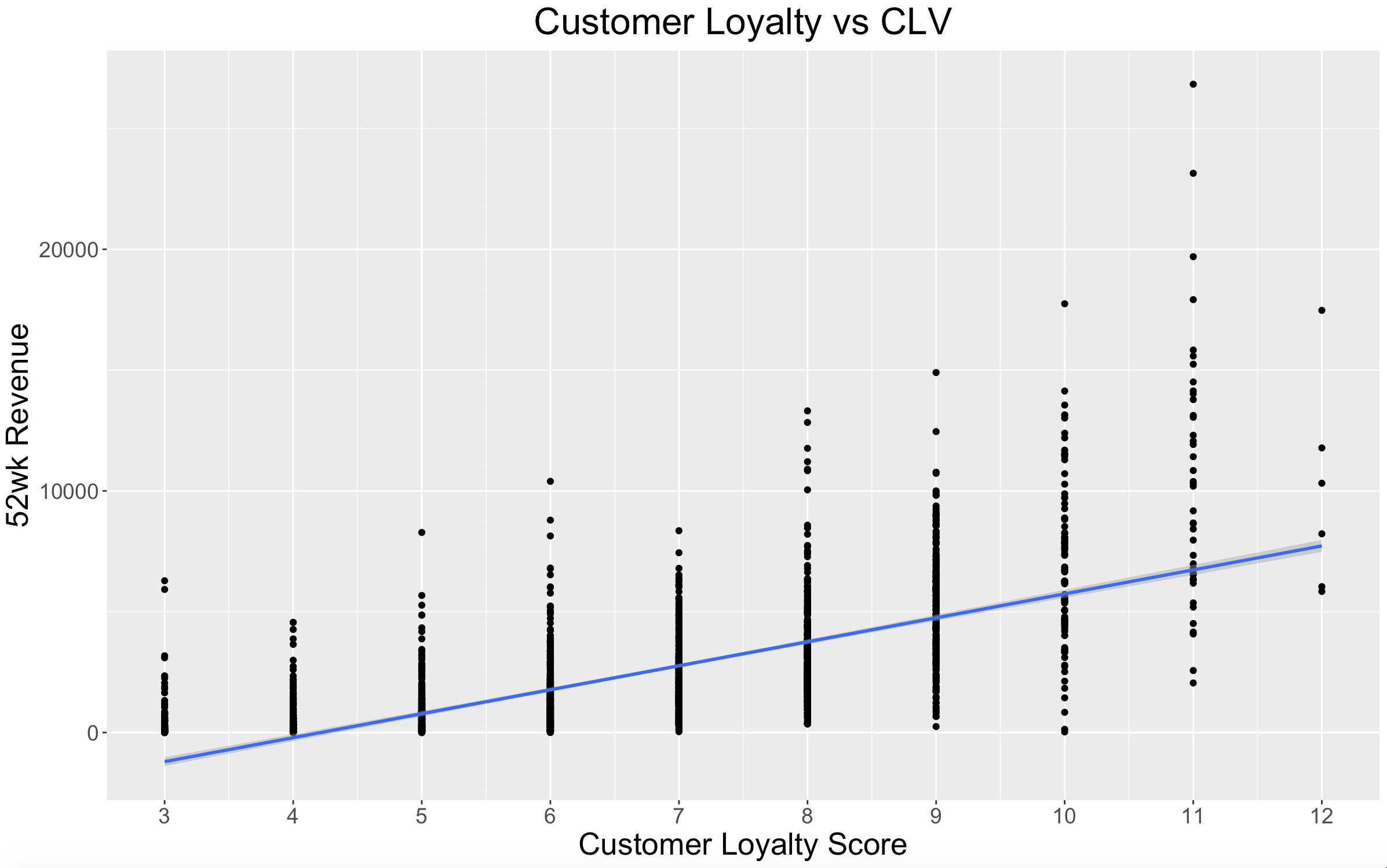
As would be expected, there is a clear positive relationship between customer loyalty scores and customer lifetime value.

The ScoreGroup column in the feature set will need to be transformed into dummy variables.

# dummy columns for score groups
dummy_cols <- dummy(customer_clv_big$ScoreGroup)
dummy_cols <- as.data.frame(dummy_cols)
customer_clv_big <- cbind(customer_clv_big,dummy_cols)

The last step before building our model is creating Customer Lifetime Value segments with our dependent variable, similar to the way we created segments for recency, frequency, and value. There will be 3 CLV segments: High-Value, Mid-Value, Low-Value.

# Define CLV segments
set.seed(1234)
clv_clusters <- kmeans(customer_clv_big$Revenue52wk, centers = 3)
customer_clv_big$clvCluster <- clv_clusters$cluster
customer_clv_big$clvCluster <- ifelse(customer_clv_big$clvCluster==3, 1,
                                      ifelse(customer_clv_big$clvCluster==1,2,3))
customer_clv_big$clvCluster <- as.factor(customer_clv_big$clvCluster)

By doing this we will have two options for a dependent variable which will allow us to build two separate CLV models. One model will predict the CLV in dollars, and the other will predict the CLV segment.

Building the Model

CLV in $$$

The first model will predict CLV in dollars. For this model, “Revenue52wk” will be used as the dependent variable.

Before splitting the data into a training and test set, the columns “household_key” and “ScoreGroup” should be dropped from our feature set (household_key is a unique identifier and ScoreGroup has been transformed into dummy variables).

# drop household ScoreGroup in feature set
customer_clv_feature <- customer_clv_big[, -which(names(customer_clv_big) %in% c("household_key","ScoreGroup","clvCluster"))]

Now we can split the feature set into a training and test set. A 75/25 split will be implemented.

set.seed(1234)
# split into test and train set
index <- createDataPartition(customer_clv_feature$Revenue52wk, p = 0.75, list = FALSE)

# training set
train_clv <- customer_clv_feature[index, ]

# test set
test_clv <- customer_clv_feature[-index, ]

With the training and test sets now established, we can start building and comparing different models via the caret package. I will compare the performances of random forest, multiple linear regression, and neural network models.

train_control <- trainControl(method="repeatedcv", repeats=3)

# Train a model
model_clv <- train(train_clv[, -which(names(train_clv) %in% c("Revenue52wk"))],
                   train_clv[, "Revenue52wk"],
                   method = 'lm',
                   family = "response",
                   trControl = train_control)

(Above is the code for building the multiple linear regression model, which performed the best. I’ll go into further detail on performances in the Results section.)

CLV Segments

The second model will predict CLV segments by using “clvCluster” as the dependent variable. The code for building this model is very similar to the first model. Since this is a classification model rather than regression, I will compare performances across xgBoost, random forest, k-nearest neighbors, and neural network models.

# drop household ScoreGroup in feature set
customer_clv_clust_feature <- customer_clv_big[, -which(names(customer_clv_big) %in% c("household_key","ScoreGroup","Revenue52wk"))]

set.seed(1234)
# split into test and train set
index <- createDataPartition(customer_clv_clust_feature$clvCluster, p = 0.75, list = FALSE)

# training set
train_clv_clust <- customer_clv_clust_feature[index, ]

# test set
test_clv_clust <- customer_clv_clust_feature[-index, ]

train_control <- trainControl(method="repeatedcv", repeats=3)

# Train a model
model_clv_clust <- train(train_clv_clust[, -which(names(train_clv_clust) %in% c("clvCluster"))],
                         train_clv_clust[, "clvCluster"],
                         method = 'xgbTree',
                         trControl = train_control)

(Above is the code for building the neural network model, which performed the best.)

Results

CLV in $$$

Model performance for predicting CLV in dollars:

Model	RMSE	R-squared
Random Forest	$1619.71	0.64
Multiple Linear Regression	$1514.14	0.68
Neural Network	$1520.01	0.68

I selected the multiple linear regression model because it just slightly outperformed the neural network.

Here is how the model did with predicting on the test set.

predictions_clv <- predict(object = model_clv,
                           test_clv[, -which(names(test_clv) %in% c("Revenue52wk"))])
actuals_preds <- data.frame(cbind(actuals=test_clv$Revenue52wk, predicteds=predictions_clv))
correlation_accuracy <- cor(actuals_preds)
correlation_accuracy[1,2]^2
rmse(test_clv$Revenue52wk, predictions_clv)

The model had an RMSE of $1482.27 and an R-squared of 0.66 on the test set dataset.

CLV Segments

Model performance for predicting CLV segments:

Model	Accuracy
xgBoost	0.81
Random Forest	0.80
K-Nearest Neighbors	0.79
Neural Network	0.81

The xgBoost model and neural network had the same accuracy on the training set. However, I selected the neural network model because it performed better on the test set.

Here is how the model did with predicting on the test set.

predictions_clv_clust <- predict(model_clv_clust,test_clv_clust[, -which(names(test_clv_clust) %in% c("clvCluster"))])

confusionMatrix(predictions_clv_clust,test_clv_clust$clvCluster)

The neural network model had an accuracy of 0.80 on the test set. In terms of sensitivity, predicting Low-Value customers was 0.93, Mid-Value was 0.59, and High-Value was 0.53. (The xgBoost model also had an accuracy of 0.80 on the test set, but its sensitivity was noticeably worse.)

What’s Next?

Now that we have a way of identifying our customers with high lifetime value, we are going to want to make sure that we retain them. So, next we will build a model to predict which customers are in danger of churning.